#*******************
#* Global model
#*******************
code <- nimbleCode({
# Priors and constraints
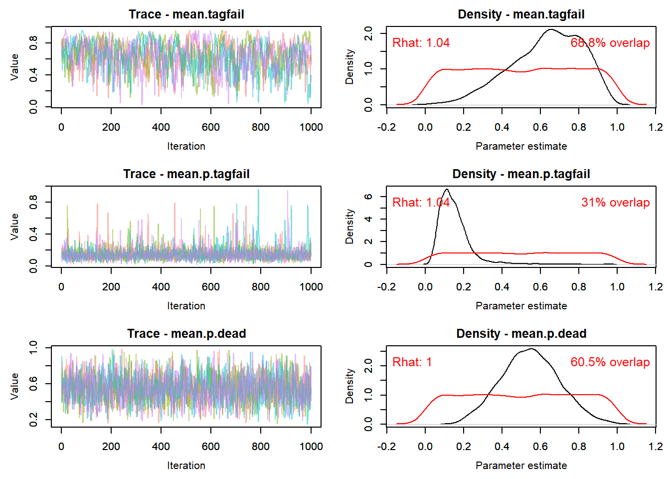
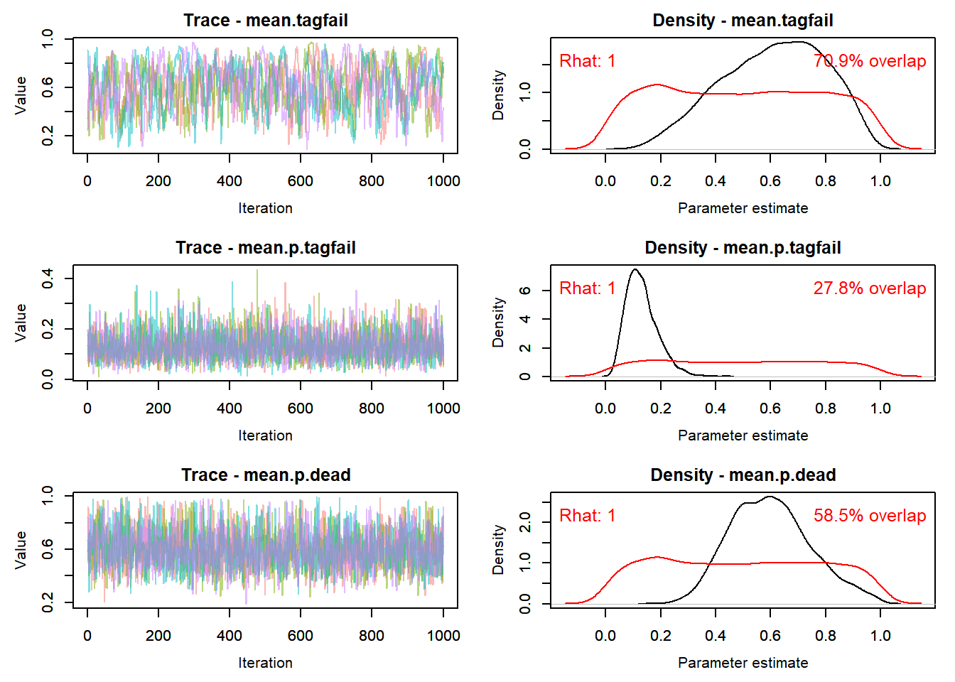
mean.p.dead ~ dbeta(1, 1) # uninformative prior for monthly probabilities
l.p.dead <- logit(mean.p.dead) # logit transformed intercept
mean.tagfail ~ dbeta(1, 1) # uninformative prior for monthly probabilities
l.tagfail <- logit(mean.tagfail) # logit transformed intercept
mean.p.tagfail ~ dbeta(1, 1) # uninformative prior for monthly probabilities
l.p.tagfail <- logit(mean.p.tagfail) # logit transformed intercept
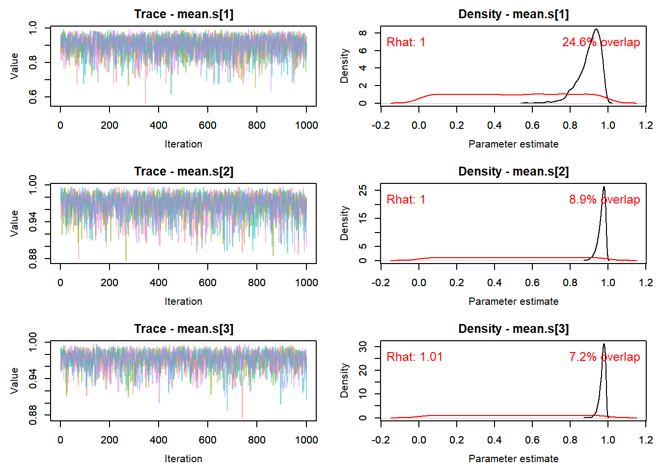
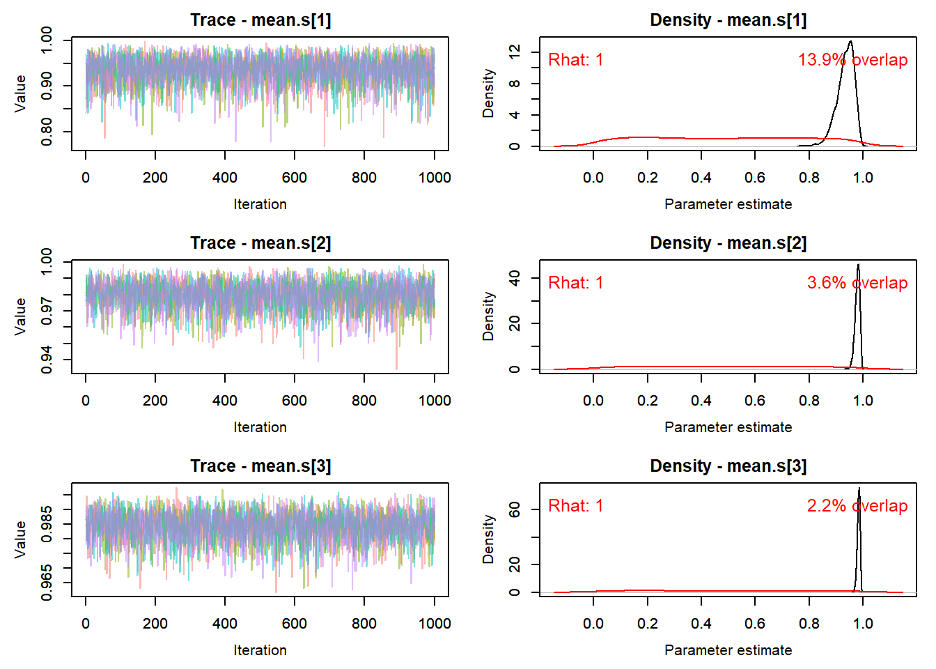
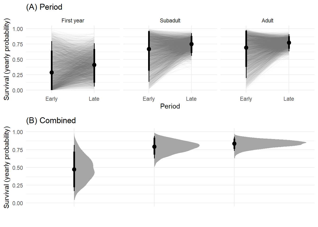
for (x in 1:3){
mean.s[x] ~ dbeta(1, 1) # uninformative prior for monthly probabilities
l.s[x] <- logit(mean.s[x])
}# xx logit transformed survival intercept
for (xx in 1:3){
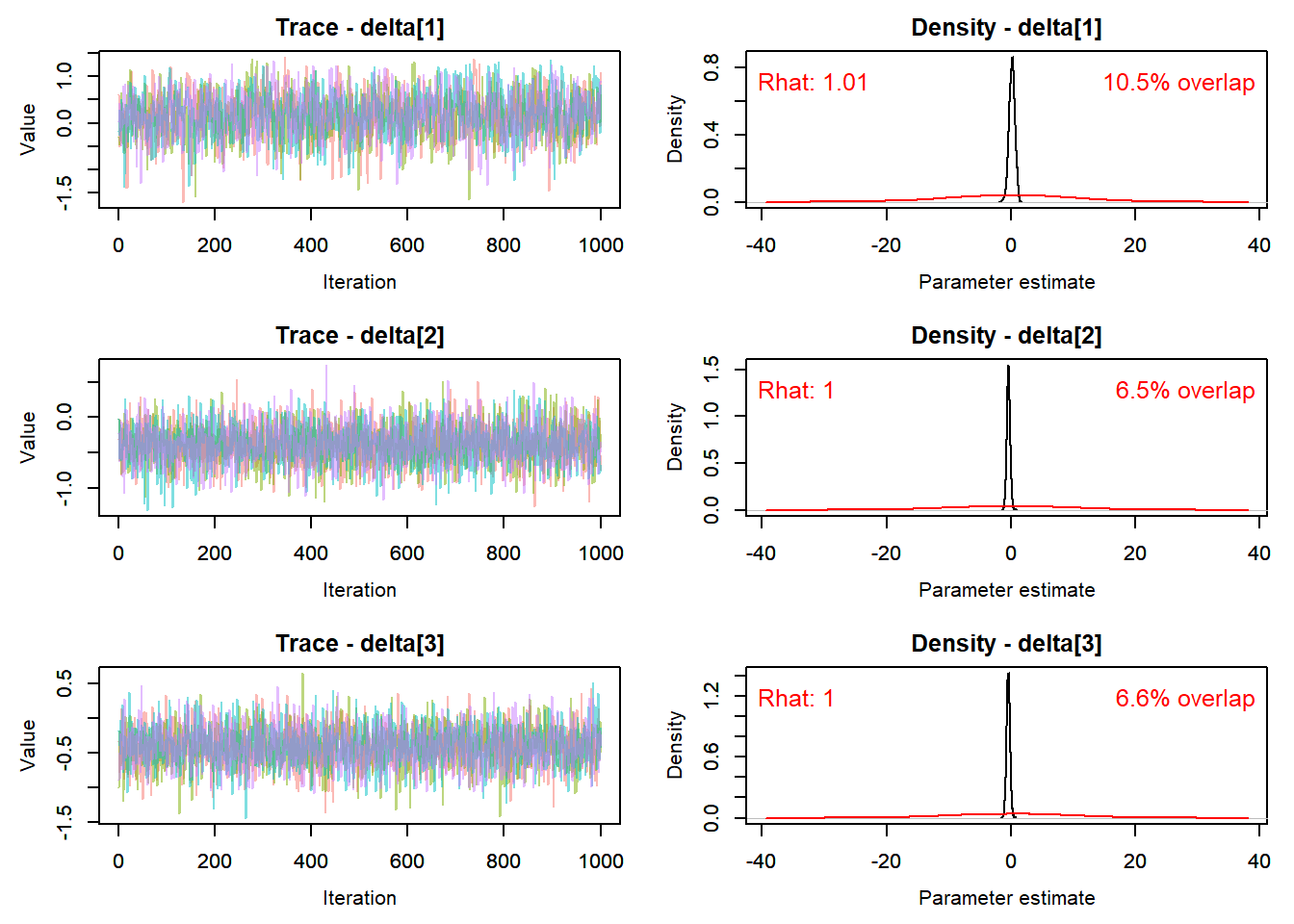
delta[xx] ~ dnorm(0, sd=10) # covariates for survival
} # x
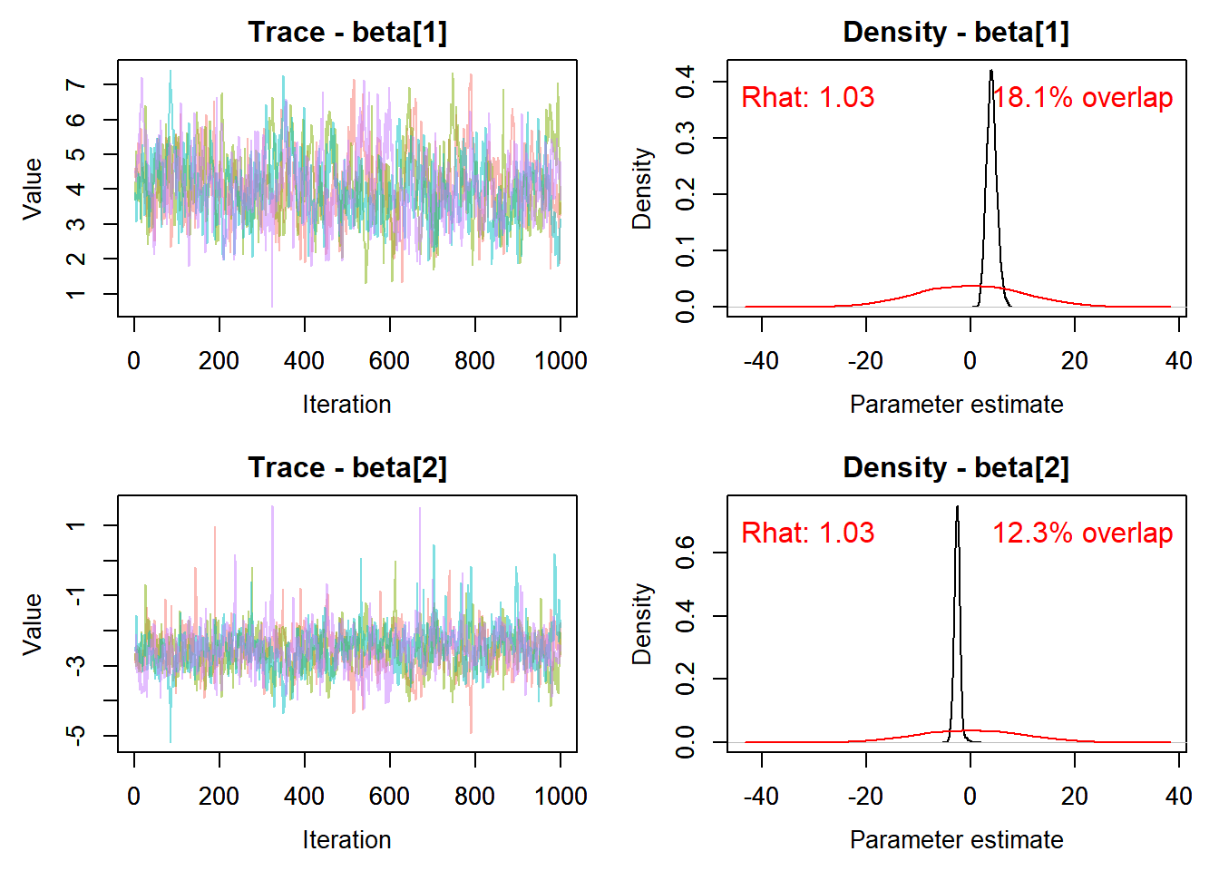
for (xxx in 1:2){
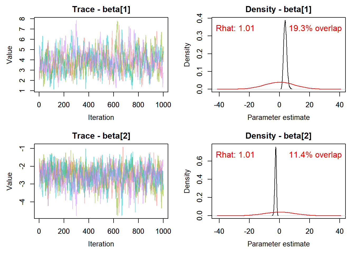
beta[xxx] ~ dnorm(0, sd=10) # covariates for tagloss
} # xxxx
# ages 0,1,2,3,4,5,6
alpha[1:7] <- c(1,1,1,1,1,1,1)
pi[1,1:7] ~ ddirch(alpha[1:7])
pi[2,1] <- 0
pi[2,2:6] ~ ddirch(alpha[2:6])
pi[2,7] <- 0
#### MONTHLY SURVIVAL PROBABILITY
for (i in 1:nind){
first_age[i] ~ dcat(pi[known[i],1:7])
for (t in f[i]:(ntime-1)){
# translate to age classes:
# 0 year old = 1,
# 1-5 year old subadult = 2-6
# and >=6 year old adult = 7
age[i,t] <- ( (first_age[i]-1) + t/12 - f[i]/12 )
age.class[i,t] <- ifgreaterFun( age[i,t], 1, 6 )
logit(s[i,t]) <- l.s[ age.class[i,t] ] +
delta[1]*c(-1, 1)[ period.cat[t] + 1 ] +
delta[2]*c(-1, 1)[ rehabbed[i] + 1 ] +
delta[3]*c(-1, 1)[ sp[i] + 1 ]
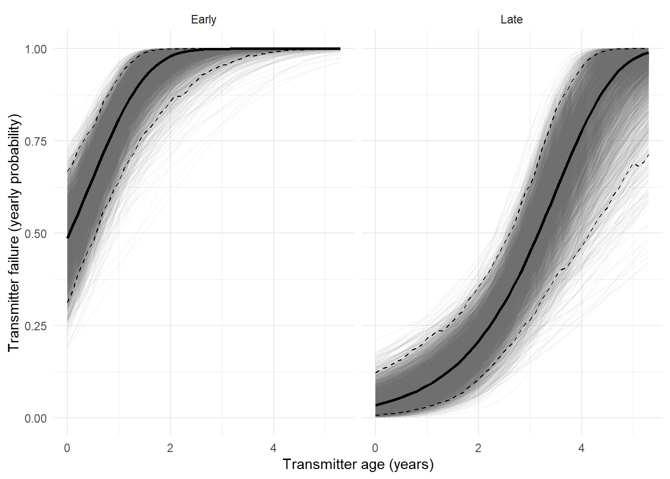
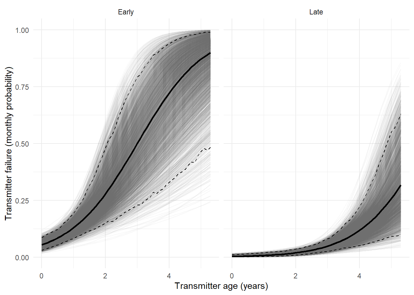
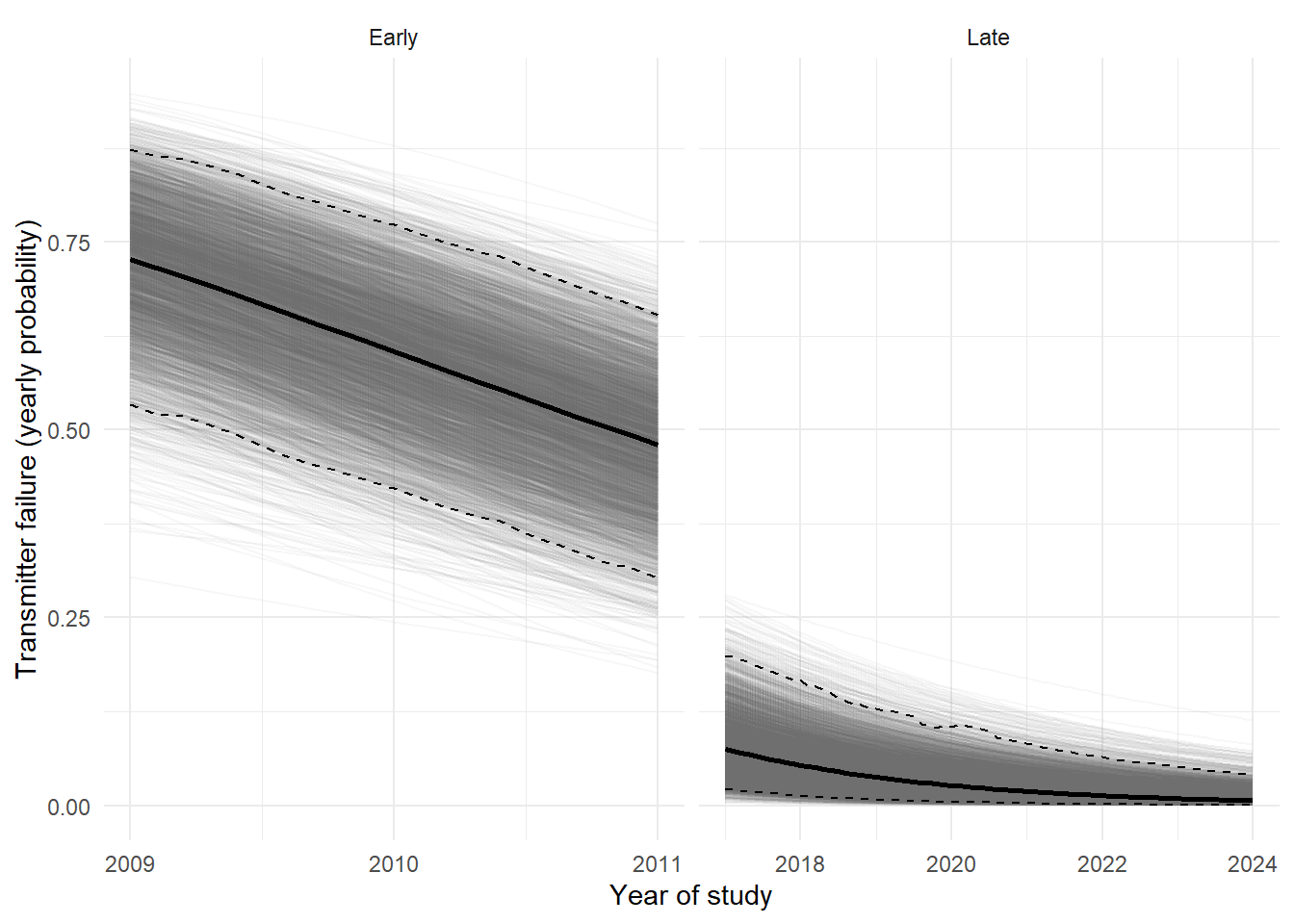
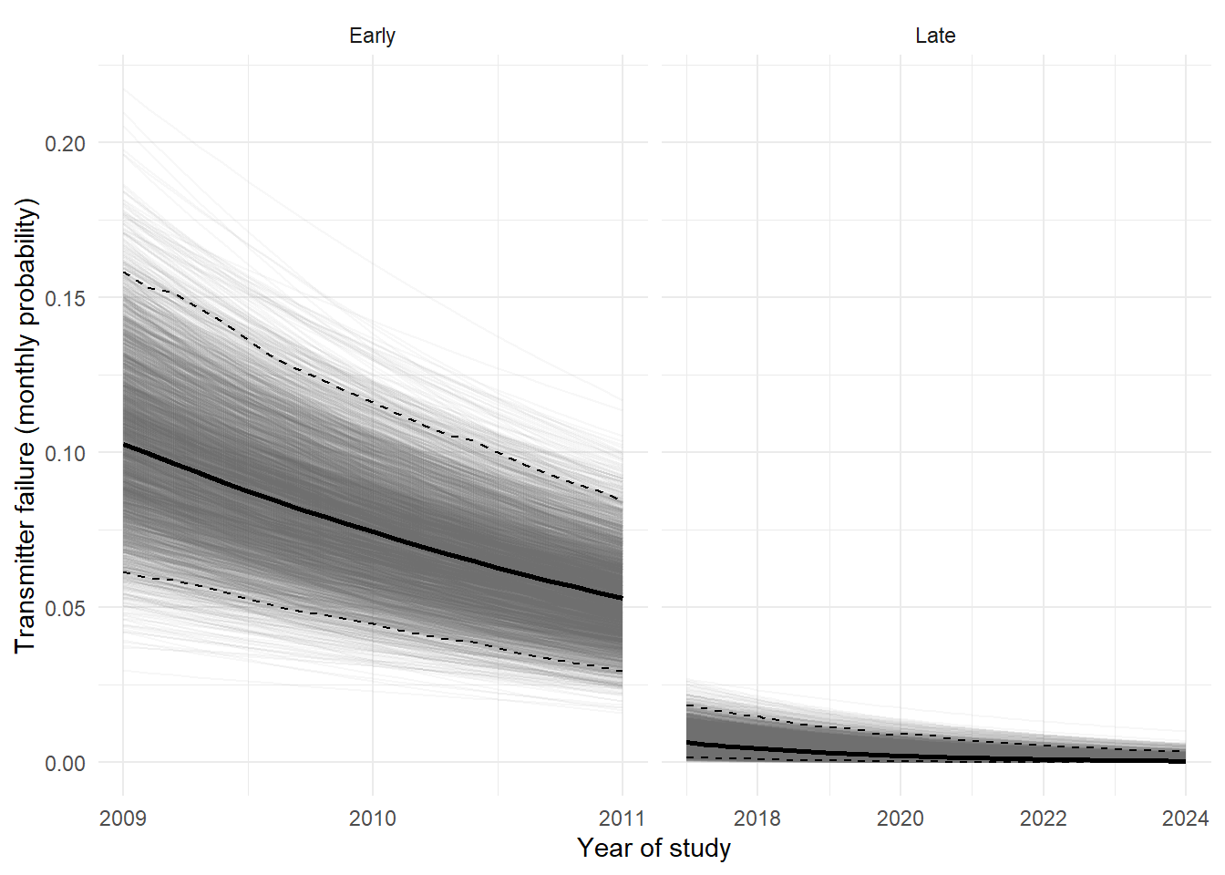
logit(tagfailed[i,t]) <- l.tagfail +
beta[1]*tag.age.sc[i,t] +
beta[2]*year.cont[t]
logit(p.tagfailed[i,t]) <- l.p.tagfail # prob of detecting tag failure
logit(p.dead[i,t]) <- l.p.dead # probability of dead recovery
} #t
} #i
# Define state-transition and observation matrices
for (i in 1:nind){
for (t in f[i]:(ntime-1)){
# Define probabilities of state S(t+1) [last dim] given S(t) [first dim]
ps[i,1,1,t]<-(1-tagfailed[i,t])*s[i,t]
ps[i,1,2,t]<-tagfailed[i,t]*s[i,t]
ps[i,1,3,t]<-(1-tagfailed[i,t])*(1-s[i,t])
ps[i,1,4,t]<-tagfailed[i,t]*(1-s[i,t])
ps[i,2,1,t]<-0
ps[i,2,2,t]<-1
ps[i,2,3,t]<-0
ps[i,2,4,t]<-0
ps[i,3,1,t]<-0
ps[i,3,2,t]<-0
ps[i,3,3,t]<-1
ps[i,3,4,t]<-0
ps[i,4,1,t]<-0
ps[i,4,2,t]<-0
ps[i,4,3,t]<-0
ps[i,4,4,t]<-1
# Define probabilities of O(t) [last dim] given S(t) [first dim]
po[i,1,1,t]<-1
po[i,1,2,t]<-0
po[i,1,3,t]<-0
po[i,1,4,t]<-0
po[i,1,5,t]<-0
po[i,2,1,t]<-0
po[i,2,2,t]<-p.tagfailed[i,t]
po[i,2,3,t]<-0
po[i,2,4,t]<-0
po[i,2,5,t]<-(1-p.tagfailed[i,t])
po[i,3,1,t]<-0
po[i,3,2,t]<-0
po[i,3,3,t]<-p.dead[i,t]
po[i,3,4,t]<-0
po[i,3,5,t]<-(1-p.dead[i,t])
po[i,4,1,t]<-0
po[i,4,2,t]<-p.tagfailed[i,t]*(1-p.dead[i,t])
po[i,4,3,t]<-(1-p.tagfailed[i,t])*p.dead[i,t]
po[i,4,4,t]<-p.tagfailed[i,t]*p.dead[i,t]
po[i,4,5,t]<-(1-p.tagfailed[i,t])*(1-p.dead[i,t])
} #t
} #i
# Likelihood
for (i in 1:nind){
y[i, (f[i] + 1):last[i]] ~
dDHMMo(init = ps[i, y.first[i], 1:4, f[i]],
probObs = po[i, 1:4, 1:5, f[i]:(last[i] - 1)],
probTrans = ps[i, 1:4, 1:4, (f[i] + 1):(last[i] - 1)],
len = last[i] - f[i],
checkRowSums = 0)
} #i
} ) # nimbleCode
inits <- function(){ list(beta = rnorm(2,0,0.5),
delta = rnorm(3,0,0.5),
mean.s = runif(3,0,1),
mean.tagfail = runif(1),
mean.p.tagfail = runif(1),
mean.p.dead = runif(1),
alpha = rep(1/7, 7),
first_age = ifelse(is.na(datl$first_age), 3, NA)
)}
run <- function(seed, datl, constl, code, inits){
library('nimble')
library('nimbleEcology')
source("R/functions.R")
pars <- c( "beta",
"delta",
"mean.s", "mean.tagfail", "mean.p.tagfail", "mean.p.dead",
"l.s", "l.tagfail", "l.p.tagfail", "l.p.dead",
"logProb_y", "first_age", "pi")
nimbleOptions(showCompilerOutput= TRUE)
mod <- nimbleModel(code, calculate=T,
constants = constl,
data = datl,
inits = inits,
buildDerivs = FALSE)
cmod <- compileNimble( mod )
conf <- configureMCMC(cmod, monitors=pars, print = TRUE, enableWAIC = TRUE)
mc <- buildMCMC(conf, project=cmod)
cmc <- compileNimble(mc, project=cmod, showCompilerOutput = TRUE)
printErrors()
nc <- 1; nt <- 20; ni <- 100000; nb <- 80000
post <- runMCMC(cmc,
niter = ni,
nburnin = nb,
nchains = 1,
thin = nt,
samplesAsCodaMCMC = T,
setSeed = seed,
WAIC = TRUE)
return(post)
} # run model function end
this_cluster <- makeCluster(4)
post <- parLapply(cl = this_cluster,
X = 1:4,
fun = run,
datl = datl,
constl = constl,
code = code,
inits = inits())
stopCluster(this_cluster)
save(post, datl, code,
file="outputs/gyps-28Apr2026-marginalized-global.RData")